In Journey to a Black Hole, I trace a ray backward from the camera for each astronomical pixel. Its path determines what ends up there: the sky, light from the disk, or black where the ray is captured.
This is how the Schwarzschild version works, from the camera ray through to the final pixels. The WGSL examples below are shortened pieces of the renderer. The linked source has the imports, bindings and complete Bevy setup.
Run the reference
The project uses Rust and Bevy 0.19.1. These examples follow commit bd964932. With Rust 1.95 or newer installed:
git clone https://github.com/furkanmamuk/journey-to-a-black-hole.git
cd journey-to-a-black-hole
git checkout bd964932ee1751ea65e2cb2c403cbd50589b0468
cargo run --release --locked -- --preset 2
The tested setup is Windows/Vulkan on an RTX 4060. Other hardware and backends are unverified, and this revision has no playable browser build. There’s also a Windows download on itch.io.
Keep Schwarzschild selected. Press F2 to hide the disk, F7 to remove the quantized presentation, and G to show the celestial grid. That gives you a clear view of the lensing while working on the ray calculation.
Units and coordinates
All positions in the calculation are relative to the black hole. Subtract its world position from the camera position before tracing.
I use geometrized units:
G = c = 1
rs = 2M
rs is the Schwarzschild radius; M is mass expressed as a length. Setting rs = 1 makes the scene easier to work with. A camera at radius 20 is then twenty Schwarzschild radii away. In physical units, rs = 2GM/c².
- The event horizon is at
r = rs - The circular photon orbit is at
r = 1.5rs - The innermost stable circular orbit for disk matter is at
r = 3rs
In the code, x is position, r = length(x), and v = dx/dlambda. These are areal Cartesian coordinates: r is the Schwarzschild areal radius, although physical distances in this geometry aren’t globally Euclidean.
lambda is the affine parameter along the ray. It isn’t camera time or photon proper time. With the magnitude of conserved photon energy normalized to one, a step in lambda has length units. The math notes use the same convention.
From a pixel to a ray
The fullscreen shader turns each fragment’s UV coordinate into a direction using the camera basis:
fn camera_ray(
    uv: vec2<f32>,
    forward: vec3<f32>,
    right: vec3<f32>,
    up: vec3<f32>,
    aspect: f32,
    tan_half_fovy: f32,
) -> vec3<f32> {
    let q = uv * vec2<f32>(2.0, -2.0) + vec2<f32>(-1.0, 1.0);
    return normalize(
        forward
        + right * q.x * aspect * tan_half_fovy
        + up * q.y * tan_half_fovy
    );
}
forward points into the scene. The basis vectors are orthonormal, aspect is width divided by height, and tan_half_fovy is the tangent of half the vertical field of view. The UV origin here is at the top left; change the vertical sign if your pass uses a different convention.
You can already use this direction to sample a cubemap or a celestial grid. The stars should stay fixed in world direction as the camera rotates. My sky shader generates deterministic stars in overlapping directional charts. The fragment entry point shows how the camera ray reaches that lookup.
Before integrating, the local camera direction needs a coordinate conversion. For a static observer outside the horizon:
er = x / r
mu = dot(d, er)
f0 = 1 - rs / r0

v = mu er + (d - mu er) / sqrt(f0)
d is the unit camera direction, r0 is the observer’s radius, and er points radially outward. The conversion keeps the radial part and scales the tangential part by 1/sqrt(f0):
struct RayState {
    x: vec3<f32>,
    v: vec3<f32>,
}

// Preconditions: d is a unit local direction; r0 > rs > 0.
fn initial_state(x: vec3<f32>, d: vec3<f32>, rs: f32) -> RayState {
    let r0 = length(x);
    let er = x / r0;
    let mu = dot(d, er);
    let f0 = 1.0 - rs / r0;
    let v = mu * er + (d - mu * er) / sqrt(f0);
    return RayState(x, v);
}
Don’t normalize v afterward. It’s a coordinate derivative, and its magnitude carries the affine normalization used by the equations. The camera must also stay outside the horizon. In this renderer, moving it gives a sequence of static-observer views; the calculation doesn’t include a boost for the camera’s physical velocity or the resulting aberration.
Following the curve
The Schwarzschild spatial null-orbit equation is:
L = cross(x, v)
L2 = dot(L, L)

dx/dlambda = v
dv/dlambda = -(3/2) rs L2 x / r^5
L is conserved angular momentum per unit normalized photon energy, with length units. Calculate L2 once from the initial state.
This equation comes from the radial null constraint:
vr^2 + (1 - rs/r) L2/r^2 = 1
vr = dot(x, v) / r
Differentiating gives a centrifugal term and a relativistic correction. The centrifugal term cancels when written as Cartesian vector acceleration, leaving:
// Evaluate only on the supported exterior ray path.
fn acceleration(x: vec3<f32>, l2: f32, rs: f32) -> vec3<f32> {
    let r2 = dot(x, x);
    return -1.5 * rs * l2 * x / (r2 * r2 * sqrt(r2));
}
For a radial ray, L2 = 0. Its spatial path stays straight, including when it heads inward and is captured. The full shader adds a denominator guard to this helper.
I use second-order velocity Verlet for the Schwarzschild path. It advances position, evaluates the acceleration there, then updates velocity:
a0 = acceleration(x)
x1 = x + h v + (h^2 / 2) a0
a1 = acceleration(x1)
v1 = v + (h / 2) (a0 + a1)
fn verlet_step(y: RayState, h: f32, l2: f32, rs: f32) -> RayState {
let a0 = acceleration(y.x, l2, rs);
let x1 = y.x + h * y.v + 0.5 * h * h * a0;
let a1 = acceleration(x1, l2, rs);
let v1 = y.v + 0.5 * h * (a0 + a1);
return RayState(x1, v1);
}The calling loop has to keep these steps safe. Bound or shorten h so the trial endpoint stays outside the horizon before evaluating a1. Checking only the old position isn’t enough.
A small fixed step is fine for an initial version at a modest camera distance. The project’s distance-dependent rule starts with:
h = step_scale * min(0.16r, 0.12r^2 / (sqrt(L2) + 0.01))It then clamps h and caps spatial displacement using length(v). The 0.01 is a numerical regularizer in scene units. This is a heuristic: it has no local error estimate, and the fixed minimum step eventually limits further refinement. Use the complete step policy, including its caps, when comparing with the demo.
The trace loop, in pseudocode:
state = initial_state(camera_position, camera_direction)
L2 = squared_length(cross(state.x, state.v))

repeat up to the step budget:
    if the affine-distance budget is exhausted:
        return UNFINISHED
    if radius is inside the capture threshold:
        return CAPTURED
    if outside the escape radius and moving outward:
        return SKY(normalize(state.v))

    choose a step
    next = verlet_step(state, step, L2)
    test the segment for a disk event
    state = next

return UNFINISHED
Capture stops at 1.015rs, a numerical safety margin outside the horizon. Escape requires both a sufficiently large radius and outward motion. At that point, a normalized copy of v supplies the sky direction. Keep the original velocity unnormalized during integration.
The project allows at most 768 steps. Difficult rays can still exhaust that budget, so the result keeps “unfinished” separate from “captured.” F11 displays unfinished rays in magenta; in the normal image they’re black and can be mistaken for part of the shadow.
Disk intersections
The disk is a thin annulus through the origin with unit normal n. For Schwarzschild, start its inner edge at 3rs. A constant bright colour is enough to check the shape before adding emission.
Most rays cross the disk between integration samples. Compare the signed plane distances at the ends of each step:
d0 = dot(old_position, n)
d1 = dot(new_position, n)

if d0 and d1 have opposite signs:
    t = d0 / (d0 - d1)
    hit = mix(old_position, new_position, t)
Accept the hit when inner_radius < length(hit) < outer_radius. Guard the denominator and use a consistent half-open crossing rule so a hit exactly at an endpoint isn’t counted twice.
Linear interpolation works for short segments. The project’s event calculation instead uses cubic Hermite interpolation from the endpoint positions and velocities, followed by ten bisection iterations.
Both methods still need a bracketed crossing. A large step can cross the plane twice and leave its endpoints on the same side. Grazing rays need care too, and an exactly coplanar ray is singular for this zero-thickness model. Check tilted views with smaller steps and keep the camera slightly above the disk plane.
An opaque disk can stop the trace at its first valid hit. Mine accumulates emission with approximate transmission 0.04 per crossing, stopping after two emitting crossings leave negligible transmission. The result is a thin emitting surface with no volumetric plasma calculation.
Moving sideways now changes which parts of the disk the rays reach. Some appear above and below the dark centre:
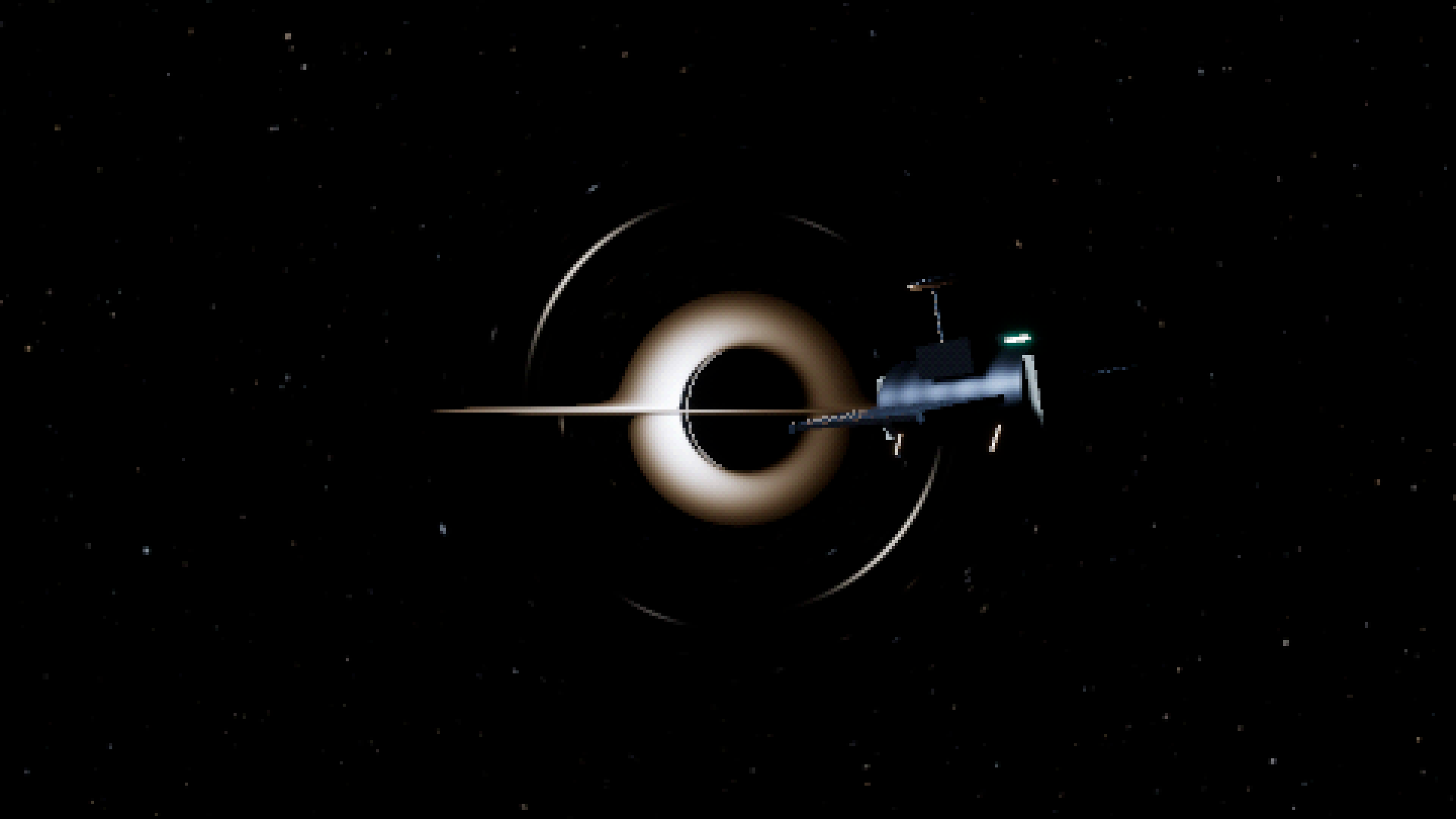
Disk emission
The disk’s radial profile is:
F(r) = (r_in/r)^3 (1 - sqrt(r_in/r))
T(r) = T_scale * F(r)^(1/4)
F is dimensionless relative bolometric flux, r_in is the inner radius, and T_scale is in kelvin. The default is 18,000 K. The zero-torque factor brings the flux to zero at the inner edge, with a peak farther out.
This is a simplified Newtonian no-torque profile. The temperature scale is adjustable; it isn’t inferred from mass and accretion rate. A full relativistic disk model would need a different flux calculation.
The spectral shader samples the Planck spectrum at 41 wavelengths from 380 to 780 nm, integrates against CIE colour-matching functions, then converts XYZ to linear sRGB. It uses this spectral shape:
B(lambda, T) ∝ 1 / [lambda^5 (exp(14387.76877 / (lambda T)) - 1)]Here lambda is wavelength in micrometres, distinct from the affine parameter, and T is in kelvin. Physical constants and the common wavelength interval are absorbed into the normalization. The colour stays in linear HDR. The CIE table has its own attribution and licence, which need to stay with the data if you reuse it.
Redshift and orbital motion
Gravity and the disk’s motion change the frequency reaching the observer. For the Schwarzschild disk:
M = rs / 2
Omega = sqrt(M / r^3)
ut = 1 / sqrt(1 - 3M/r)
L_n = dot(n, cross(hit_position, hit_velocity))
f0 = 1 - rs/r0

g = 1 / [sqrt(f0) ut (1 + Omega L_n)]
Omega is the circular emitter’s angular velocity in coordinate time. ut, usually written u^t, is the contravariant time component of its four-velocity. L_n is the ray’s signed angular momentum about the disk normal. The frequency ratio g is observed divided by emitted, so values above one give a blueshift.
The plus sign in 1 + Omega L_n comes from tracing backward. With metric signature (-,+,+,+), the backward ray has conserved covariant time momentum p_t = +1. A formula using forward photon momentum needs its sign converted before it can be used here.
The u^t factor includes transverse Doppler shift alongside the gravitational contribution. The implementation also handles spin; these equations set it to zero.
Thermal emission is seen at temperature gT. Bolometric intensity transforms with g^4; frequency-specific intensity uses g^3 with a shifted frequency argument. The disk’s thermal_rgb function divides its colour integral by T^4, giving colour per unit relative bolometric flux:
// thermal_rgb must have the repository's per-bolometric-flux normalization.
let observed_temperature = emitted_temperature * g;
let colour = thermal_rgb(observed_temperature)
    * relative_flux
    * pow(g, 4.0)
    * artistic_hdr_scale;
That normalization matters. If your colour function returns a full, unnormalized Planck intensity at gT, another multiplication by g^4 counts the energy shift twice. The final shader also applies edge tapering and an artistic HDR brightness scale.
The Bevy pass
On the Rust side, the uniform struct uses ShaderType and Vec4 fields to match the WGSL layout. Check alignment if you change that layout, especially around three-component vectors.
The render pass reads the existing HDR scene, its depth texture and the settings buffer. It draws a fullscreen triangle into an Rgba16Float target before later post-processing.
Foreground pixels are preserved. The shader traces only where depth is zero, meaning uncovered background in Bevy’s reverse-depth convention. Check that convention if you’re porting this to another engine.
The probe therefore keeps its ordinary perspective projection. It isn’t lensed or hidden by the black hole. Supporting that would require intersections with foreground geometry along the curved rays; the existing depth texture only contains the objects’ ordinary camera projection.
The pixel treatment
The coarse presentation comes after the HDR scene:
HDR scene and geodesic background
    → bloom and exposure
    → tone mapping
    → area reduction
    → tonal quantization and ordered dither
    → nearest-neighbour expansion
    → UI
By default, I render HDR at 960×540 and reduce it to a 480×270 presentation grid before enlarging it. The reduction shader averages the covered source area with overlap weights, including fractional pixel coverage. This reduces flicker in thin bright features compared with picking one source sample per cell.
Tonal quantization rounds perceptual channel values to a configurable number of levels. A fixed 4×4 Bayer pattern spreads the rounding error across the presentation grid, and nearest-neighbour expansion keeps the cells sharp. Keep the dither pattern stable between frames.
F7 bypasses this treatment. It helps separate changes in the ray calculation from those introduced by tone mapping and downsampling.
Checking the result
With disk and bloom disabled, track the null constraint along each ray:
residual = abs(vr^2 + (1 - rs/r) L2/r^2 - 1)It should stay close to zero. The shader records a normalized version of the maximum residual encountered along the path. Compare cross(x, v) with its initial value as well, to check angular-momentum drift.
There are useful reference cases:
- Radial inward and outward rays have straight spatial paths. The inward ray reaches the capture threshold
- For an incoming ray from far away, weak-field deflection approaches
2rs/bradians, wherebis its impact parameter - The critical incoming impact parameter is
b_critical = 3sqrt(3)rs/2. Nearby rays on either side should separate into capture and escape as you refine the integration - For a static camera at
r0 > 1.5rs, the shadow half-angle satisfiessin(alpha) = b_critical sqrt(1 - rs/r0) / r0
The shadow is larger than the horizon’s Euclidean angular size, so a flat sphere of radius rs would be the wrong reference.
Compare results after halving the step scale, allowing more steps and affine distance, and increasing the escape radius. Reduce the minimum step too if it’s preventing refinement. Check disk intersections and sky directions as well as capture: a small constraint residual alone doesn’t establish accuracy near a critical ray or detect a missed disk event. The finite escape boundary also omits some remaining deflection.
The CPU reference tests use higher precision than the GPU. Passing them doesn’t certify every f32 pixel. The validation notes record the tests and native runs performed for the project.
Kerr and the remaining work
The spinning version uses a separate Kerr–Schild Hamiltonian shader. It integrates position and canonical momentum together with RK4, using analytic metric derivatives. Spin changes the horizon, the disk’s stable inner edge and the ray paths through frame dragging. The conserved angular-momentum component is the axial canonical Lz = x p_y - y p_x, rather than the full vector used above.
The disk in both versions remains an analytic surface. There is no fluid dynamics, turbulence, thickness or delayed emission history. A moving observer and curved-ray foreground visibility also need further work.
Eric Bruneton’s Real-time High-Quality Rendering of Non-Rotating Black Holes covers the geometry and local frames in more depth, with a lookup-table approach to accelerating the ray tracing. For the files behind this renderer, see the project’s architecture notes.