Furkan Mamuk
I wanted to keep looking back while falling through an event horizon. Not stop the camera at the boundary, or cut to black, but follow an observer who actually crosses it.
I used a freely falling observer in an idealized Kerr spacetime. The camera axes are parallel transported along the trajectory, so its orientation is carried along like a gyroscope’s. That gives me a horizon crossing at a definite time on the observer’s own clock, with a view just before it, right on it, and just after. In these renders, the rear sky is still there.
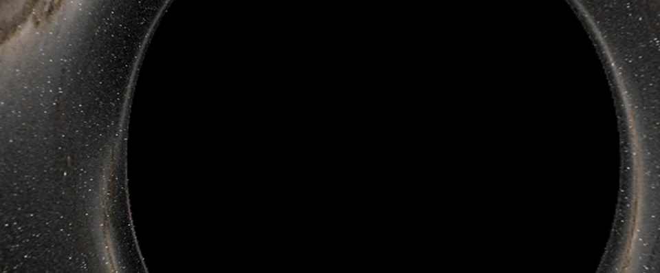
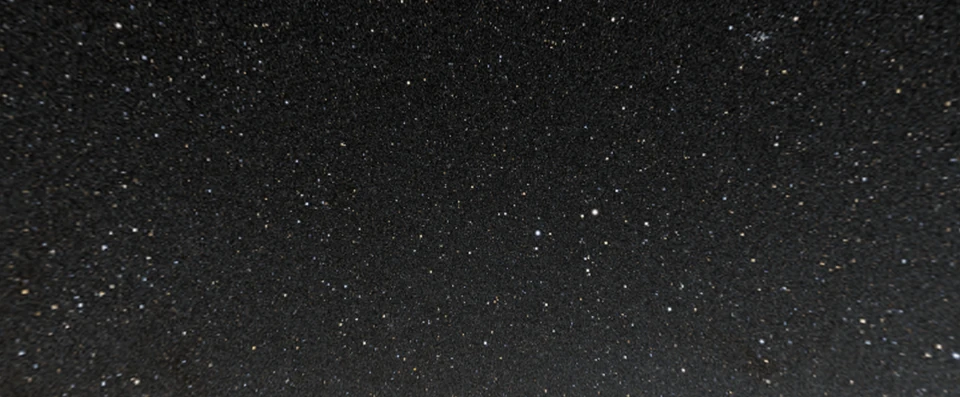
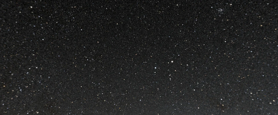
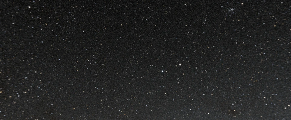
For this run I used spin +0.8 and an inclination of 65°. The seconds are based on a mass of 4.3 million solar masses. The original panoramas are 1920×960, at four rays per pixel; the forward and rear views are projections of them.
At the horizon, rays connecting to the distant sky have a frequency ratio g from 0.478 to 6.58. That’s the frequency received by the observer divided by the frequency emitted at the source. Above one is blueshift; below one is redshift.
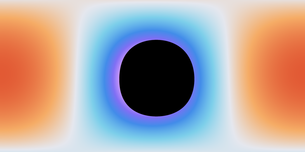
The optical sky gets its appearance from an RGB catalogue. I don’t have the source spectrum for every direction, so those pretty star colours are not a full spectral rendering of the shift. That’s why the frequency map is separate.
The optical images and the ray maps agree on sample counts and frequency ranges at all three poses, with no unresolved rays in this set.
A sky map doesn’t know where a star is
For the next experiment I moved to Sgr A* and changed what counts as a light source. A distant sky catalogue gives a ray a colour based on the direction it points. That works for the background, but a star near the Galactic Centre has a distance and an orbit. Its position changes while the light is travelling.
Now the ray has to meet the star at the right place and the right time.
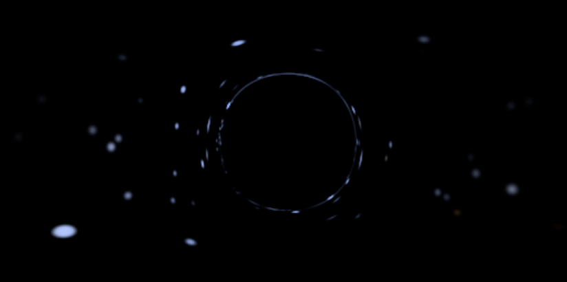
This is a separate preview with 39 finite-distance stellar orbits: four GRAVITY sources, plus 35 bound, nonoverlapping entries from Gillessen Table 3. The observer crosses the outer horizon at pose 096.
Meeting the star in the past
The offline tracer takes the observer’s frame through the horizon and traces rays backward from there. I use each ray’s lookback time to calculate the emitter’s position and velocity at the emission event. If I froze every orbit at one convenient epoch, I’d be calculating a different sky.
The output includes finite-shell intersections, frequency ratios, lookback times and spatial momenta. At the outer endpoint, the moving-source intersection uses a local-tangent approximation; I’ve checked that approximation against independent retraces. The stellar orbits themselves are propagated as Kepler ellipses from published osculating elements. I don’t want to pass either approximation off as something more elaborate.
The result is a modeled stellar sky, with some fairly specific choices behind it. Published K magnitudes are treated as approximately Ks, with an extinction correction along the line of sight from Earth. I use representative continua for the colours. The preview assumes local vacuum transfer and widened stellar sampling footprints; it leaves out diffuse emission, local dust and unresolved stars. The spin and orientation are scenario choices too.
The problem with very thin arcs
A narrow stellar image can sit between samples. One frame misses it, the next picks it up, and suddenly an arc starts blinking for no physical reason.
I didn’t want to trace a huge uniform grid through mostly empty sky. Instead I work in an annulus around the capture region and subdivide candidate cells into 3×3 where a star might contribute. It’s targeted extra sampling, not a blanket resolution increase.
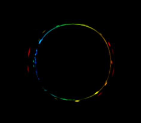
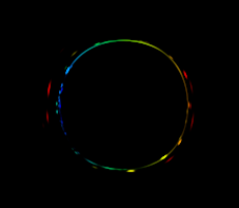
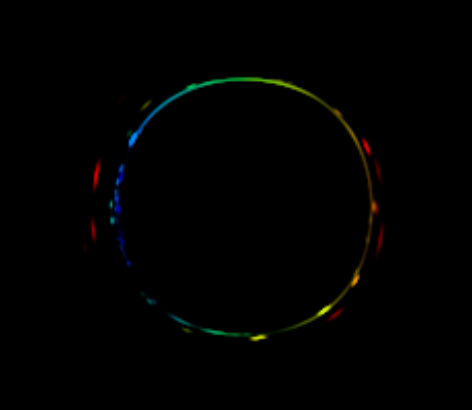
These crops isolate Ks light emitted by the stars and shifted into the visible band. They’re all shown with the same 6× display gain. The colours come from the modeled continua.
Across poses 092–102, the largest departure of integrated Ks flux from interpolation between neighbouring proper-time samples dropped from 3.2771% on the coarse grid to 0.0449% with the targeted refinement. The portfolio rounds that last value to 0.04%. This tells me the total flux changes more smoothly between poses. It doesn’t tell me every narrow arc is spatially resolved.
| Separate check | Largest reported difference | Scope |
|---|---|---|
| Independent shifted-grid preview comparison | 1.46% | Brightness-normalized Ks image at preview resolution |
| Production-width crossing comparison | 6.27% | Isolated added-stars Ks image across three poses |
The spatial checks still see differences in those thin arcs. The independent shifted-grid preview differs by as much as 1.46%; the production-width crossing comparison reaches 6.27% on the isolated added-stars Ks images. A smooth flux curve can coexist with image detail that hasn’t settled.
About the flight itself
There are 110 simulated poses, starting at 500 M and ending near 1.686 M. By the final pose, the observer has spent 3.50 seconds of proper time inside the outer horizon. I changed the playback timing to linger around the crossing, but not the ray emission times or the observer’s clock. The video contains those simulated poses; I didn’t interpolate extra frames.
Distances are in gravitational lengths, M = GM_BH/c². The scenario uses a black-hole mass of 4.297 million solar masses, which sets the conversion to seconds.
What I have here is a local preview, with a source model and a sampling strategy I can inspect. The full local Sgr A* master is still pending. Until then, the assumptions, 6× display gain and unresolved angular detail belong next to the images—not buried somewhere else.
Credits
Optical sky: Deep Star Maps 2020, NASA Goddard Space Flight Center Scientific Visualization Studio, Ernie Wright, ESA/Gaia/DPAC and the source catalogues.
Stellar inputs: GRAVITY orbital elements, GRAVITY photometry and Gillessen et al., Table 3. Colour matching: CIE 1931 2° standard observer dataset, CC BY-SA 4.0.